Generative Models
The text-to-image synthesis is the best perfect application to describe the generative models. The current best text to image synthesis is obtained through GAN, which is particularly a type of generative model. Before GAN let’s quickly summarize generative model in the below paragraph. Consider a dataset X = {x (1) , . . . , x (m) } composed of m samples where x (i) is a vector. In the particular case of this report, x (i) is an image encoded as a vector of pixel values. The dataset is produced by sampling the images from an unknown data generation distribution Pg, where r stands for real. One could think of the data generating distribution as the hidden distribution of the Universe which describes a particular phenomenon. A generative model is a model which learns to generate sample from a distribution Pg which estimates Pr. The model distribution, Pg, is a hypothesis about the true data distribution Pr. Most generative models explicitly learn a distribution Pg by maximising the expected log-likelihood Ex〜Pr log(Pg(x/θ)) with respect to θ, the parameters of the model. Intuitively, maximum likelihood learning is equivalent to putting m ore probability mass around the regions of χ with more examples from X and less around the regions with fewer examples. It can be shown that the log-likelihood maximization is equivalent to minimizing the Kullback-Leibler divergence KL(PrPg) =∫PrlogPrPgdx assuming Prand Pg are densities. One of the valuable properties of this approach is that no knowledge of the unknown Pr is needed because the expectation can be approximated with enough samples according to the weak law of large numbers.
Generative Adversarial Networks[2]
Generative Adversarial Networks (GAN) [2] are composed of two models that are alternatively trained to compete with each other. The generator G is optimized to reproduce the true data distribution Pdata by generating images that are difficult for the discriminator D to differentiate from real images. Meanwhile, D is optimized to distinguish real images and synthetic images generated by G. Overall, the training procedure is similar to a two-player min-max game with the following objective function,
min max V(D, G) = Ex〜Pdata(x) [log D(x)] + Ez〜Pz(z) [log(1- D(G(z)))] ... (1)
Where, z is a latent ”code” that is often sampled from a simple distribution (such as normal distribution). Conditional GAN is an extension of GAN where both generator and discriminator receive additional conditioning variables c, yielding G(z, c) and D(x, c). This formulation allows G to generate images conditioned on variables c.
3.1.4 Generative Adversarial Text-To-Image Synthesis[20]
Figure 1 shows the network architecture used in our project. It talks about training a deep convolutional generative adversarial network (DC-GAN) conditioned on text features. These text features are encoded by a hybrid character-level convolutional-recurrent neural network. Both the generator network G and the discriminator network D perform feed-forward inference conditioned on the text features. The encoded text description embedding is first compressed using a fully-connected layer to a small dimension followed by a leaky-ReLU and then concatenated to the noise vector z sampled in the Generator G. The following steps are the same as in a generator network in vanilla GAN; feed-forward through the deconvolutional network, generate a synthetic image conditioned on text query and noise sample.

Figure 1: Text-conditional convolutional GAN architecture[20]
GAN-CLS
The most straightforward way to train a conditional GAN is to view (text, image) pairs as joint observations and train the discriminator to judge pairs as real or fake. The discriminator has no explicit notion of whether real training images match the text embedding context. To account for this, in GAN-CLS, in addition to the real / fake inputs to the discriminator during training, a third type of input consisting of real images with mismatched text is added, which the discriminator must learn to score as fake. By learning to optimize image/text matching in addition to the image realism, the discriminator can provide an additional signal to the generator.
Algorithm[20]:
GAN-CLS training algorithm with step size
α, using mini-batch SGD for simplicity.
Input: mini-batch images x, matching text t, mis-matching t̂, number of training batch steps S
for n = 1 to S do
h ← φ(t) {Encode matching text description}
ĥ ← φ( t̂) {Encode mis-matching text description}
z ∼ N (0, 1)z {Draw sample of random noise}
x̂ ← G(z, h) {Forward through generator}
Sr ← D(x, h) {real image, right text}
Sw ← D(x, ĥ) {real image, wrong text}
Sf← D(x̂, h) {fake image, right text}
LD ← log(Sr) + (log(1 − Sw) + log(1 − Sf))/2
D ← D − α∂LD /∂D {Update discriminator}
LG ← log(Sf)
G ← G − α∂LG /∂G {Update generator}
3. End for
GAN-INT
Papers have proved that deep networks learn representations in which interpolations between embedding pairs tend to be near the data manifold. Referencing these papers, we generated a large number of additional text embeddings by simply interpolating between embeddings of training set captions. As the interpolated embeddings are synthetic, the discriminator D does not have corresponding ”real” images and text pairs to train on. However, D learns to predict whether image and text pairs match or not.
DCGAN - Architecture
To generate high-resolution images with photo-realistic details, we propose a simple yet effective DC Generative Adversarial Networks. DCGAN is one of the most popular and successful network designs for GAN. It mainly composes of convolution layers without max pooling or fully connected layers. It uses convolutional stride and transposed convolution for the downsampling and upsampling.
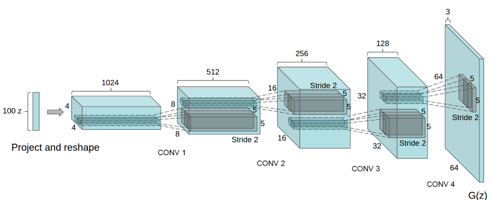
Figure 2: DCGAN – Architecture [27]
DCGAN processes:
Replace all max pooling with convolutional stride
Use transposed convolution for upsampling.
Eliminate fully connected layers.
Use Batch normalization except the output layer for the generator and the input layer of the discriminator.
Use ReLU in the generator except for the output which uses tanh.
Use LeakyReLU in the discriminator.
5.1.6 Text Embeddings
The text descriptions must be vectorized before they can be used in any model. These vectorizations are commonly referred to as text embeddings. Text embedding models were not the focus of this work, and that is why the already computed vectorizations by Reed et al. [20] are used. Other state-of-the-art models [18] use the same embeddings and their usage makes comparisons between models easier.
The text embeddings are computed using the char-CNN-RNN encoder proposed in [20]. The encoder maps the images and the captions to a common embedding space such that images and descriptions that match are mapped to vectors with a high inner product.

Figure 3: The char-CNN-RNN encoder maps images to a common embedding space [26]
To obtain vector representation of text description, Reed et al. [20] have proposed their own network. But we will be using Word2Vec and the already computed vectorizations by Reed et al. [20] are used.
IMPLEMENTATION
4.1 GENERATOR
In the generator, a noise vector z of dimension 128, is sampled from N (0, I). The text is passed through the function φ and the output φ(t) is then compressed to dimension 128 using a fully connected layer with a leaky ReLU activation. The result is then concatenated with the noise vector z. The concatenated vector is transformed with a linear projection and then passed through a series of deconvolutions with leaky ReLU activations until a final tensor with dimension 256×256×3 is obtained. The values of the tensor are passed through a tanh activation to bring the pixel values in the range [−1, 1].
4.1.1 Generator Training

Figure 4: Generator Training Process
The generator is a function that is applied to a sample from a latent random space and creates a synthetic realization. We assume that samples drawn from the hidden latent space are distributed according to a normal distribution.
The discriminator's role is to determine whether a sample is part of the training image dataset or from the generator. The misclassification error is computed as a binary cross-entropy criterion and the error back-propagated to improve the discriminator's ability to distinguish real and "fake" images. Then the generator is updated to improve the quality of the produced samples and "fool" the discriminator.
When sufficient image quality is obtained, training is stopped, and the discriminator may be discarded. The generator can now be used to create new samples. By providing larger latent vectors than used initially for training, larger output images can be produced.
4.1.1 Generator Architecture
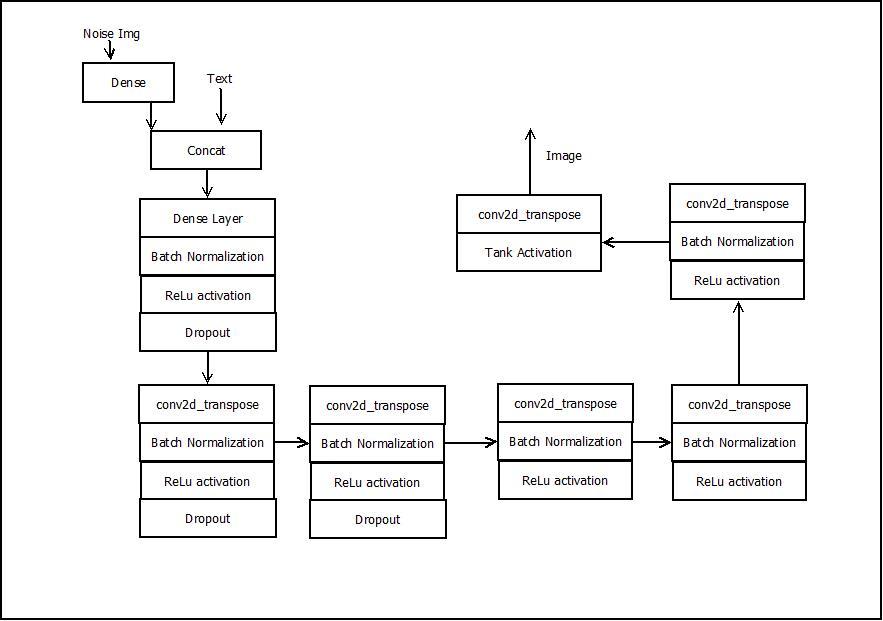
Figure 5: Generative architecture
4.2 DISCRIMINATOR
In the discriminator, the input image is passed through a series of stride 2 convolutional layers with spatial batch normalization followed by leaky ReLU. When the spatial resolution becomes 4×4, the text embeddings are compressed to a vector with 128 dimensions using a fully connected layer with leaky ReLU activations as in the generator. These compressed embeddings are then spatially replicated and concatenated 10 in depth to the convolutional features of the network. The concatenated tensor is then passed through more convolutions until a scalar is obtained. To this scalar, a sigmoid activation function is applied to bring the value of the scalar in the range [0, 1] which corresponds to a valid probability.
4.2.1 Discriminator Training

Figure 6: Discriminator training process
We train discriminator using both real images from dataset and the images generated by the generator. If the image is from dataset, the discriminator should classify it as real. If the image is from the generator, the discriminator should classify it as fake.
4.2.2 Discriminator Architecture

Figure 7: Discriminative architecture
4.3 TUNING
All models were trained with mini-batch stochastic gradient descent (SGD) with a mini-batch size of 128. All weights were initialized from a zero-centered Normal distribution with a standard deviation 0.02. In the LeakyReLU, the slope of the leak was set to 0.2 in all models. While previous GAN work has used the momentum to accelerate training, we used the Adam optimizer with tuned hyper-parameters. We found the suggested learning rate of 0.001, to be too high, using 0.0002 instead. Additionally, we found leaving the momentum term β1 at the suggested value of 0.9 resulted in training oscillation and instability while reducing it to 0.5 helped stabilize training.
4.4 PROBLEMS:
4.4.1 Hard to achieve Nash equilibrium
GAN is based on the zero-sum non-cooperative game. In short, if one wins the other loses. A zero-sum game is also called minimax. Your opponent wants to maximize its actions and your actions are to minimize them. In game theory, the GAN model converges when the discriminator and the generator reach a Nash equilibrium.
4.4.2 Low dimensional supports
Generative model distribution, Pg, lies in a low dimensional manifold, too. Whenever the generator is asked to a much larger image like 64x64 given a small dimension, such as 100, noise variable input z, the distribution of colors over these 4096 pixels has been defined by the small 100-dimension random number vector and can hardly fill up the whole high dimensional space.
4.4.3 Vanishing Gradient
If the discriminator behaves badly, the generator does not have accurate feedback and the loss function cannot represent the reality.
If the discriminator does a great job, the gradient of the loss function drops down to close to zero and the learning becomes super slow or even jammed.
4.4.4 Mode Collapse
During the training, the generator may collapse to a setting where it always produces the same outputs. This is a common failure case for GANs, commonly referred to as Mode Collapse. Even though the generator might be able to trick the corresponding discriminator, it fails to learn to represent the complex real-world data distribution and gets stuck in a small space with extremely low variety.
4.4.5 Optimization Challenges
If the generator updates are made in function space and discriminator is optimal at every step, then the generator is guaranteed to converge to the data distribution.
Unrealistic assumptions!
In practice, the generator and discriminator loss keeps oscillating during GAN training.
No robust stopping criteria in practice (unlike unlikelihood based learning)
4.4.6 No Proper Evaluation Metrics
We don’t really know when to stop the training as there is no proper evaluation metric in training GAN’s.
Visual inspection is required, a lot of people do that it when training GAN’s.
The losses don’t really tell much in GAN’s unlike other deep learning algorithms.
Due to this, often we end up not having a good GAN model.
RESULTS AND DISCUSSIONS
5.1 LOSSES
5.1.1 Ideal Case
D_loss = -log[D(x)] - log[1-D(G(z))]
G_loss = log[1-D(G(z))
So, discriminator tries to minimize D_loss and the generator tries to minimize G_loss. When GAN is trained for several steps it reaches at a point where neither generator nor discriminator can improve and D(Y) is 0.5 everywhere, Y is some input to the discriminator. In this case, when GAN is sufficiently trained to this point:
D_loss = -log(0.5) - log(1 - 0.5) = 0.693 + 0.693
G_loss = -log(0.5) = 0.693
5.1.1 With Uniform noise and SGD at discriminator and with beta = 0.05 for Adam optimizer:
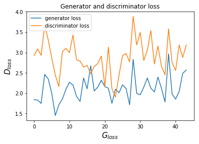
Figure 8: Generator and discriminator loss with SGD and beta = 0.05
Discriminator loss = 3.32 = 3.234 + 0.086 i.e. the Discriminator is correctly identifying real images : -log(0.039) i.e 3.9% of the time.
Generator loss = 2.501 = -log(0.082) i.e. the generator was able to fool the discriminator 8.2% time only.
Explanation:
Our aim was to minimize the generator loss and maximize the discriminator loss as per equation (1). Here we have used the random noise of uniform distribution and the generator loss was increasing as we reach 100 epochs instead of decreasing and there seems to be no improvement in the quality of image.
One of the reasons for the problem is that the discriminator got too strong relative to the generator. Beyond this point, the generator finds it almost impossible to fool the discriminator, hence the increase in it's loss. This problem is also known as vanishing gradient.
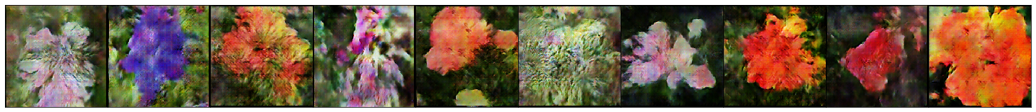
Image during training:
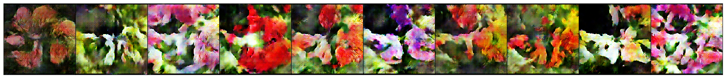
Image Generated by generator:
Text: the petals on this flower are yellow with a red center
5.1.2 Training for 100 epochs with a noise with normal distribution and adam optimizer at generator and discriminator:
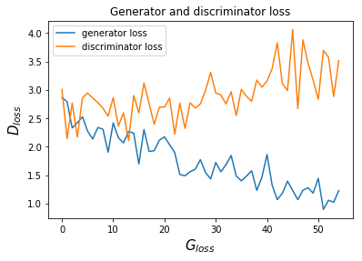
Figure 9: Generator and discriminator loss with normal distribution
Generator loss = 1.22 i.e generator is fooling discriminator by 29%
Discriminator loss = 3.51 i.e discriminator is correctly identifying real images 4.2% times only.
Generated image after training by generator:
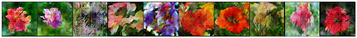
100 epochs:
Text: the petals on this flower are yellow with a red center

The image generator with this optimization was quite satisfactory as compared to other optimization performed.
Further Evaluation Metrics, Qualitative comparison, conclusions, etc were evaluated afterward.


No comments:
Post a Comment